Bayes vs. Standard Hypothesis Testing

Background

I’m going to simulate A/B test data. This could be data that’s measuring the effectiveness of a website design change or a new drug. Typically in standard inferential statistics, one would use a difference of proportions test in which the null hypothesis is that there’s no observed difference in the proportions or, if directionality of effect is important, that the effect is significant but undesirable.

In addition to this standard approach is the Bayesian approach, which is kind of more intuitive, and clearly elucidates the assumptions that went into the model.

import numpy as np
import pymc3 as pm
import scipy.stats as stats

import matplotlib.pyplot as plt
%matplotlib inline

Generate data

Repeated Bernoulli trials with known probabilities.

p_A_true = 0.28
p_B_true = 0.34

def generate_fake_data(p_A_true, p_B_true):
    n_a_points = 900
    n_b_points = 600
    a_data = stats.bernoulli.rvs(p_A_true, size=n_a_points)
    b_data = stats.bernoulli.rvs(p_B_true, size=n_b_points)
    frmt_str = "{char} observed mean: {mean} out of {n}"
    print(frmt_str.format(char='A', mean=a_data.mean(), n=n_a_points))
    print(frmt_str.format(char='B', mean=b_data.mean(), n=n_b_points))
    return a_data, b_data

a_data, b_data = generate_fake_data(p_A_true, p_B_true)

A observed mean: 0.293 out of 900
B observed mean: 0.356 out of 600

Typical approach

The typical approach to this problem is to test the null hypothesis, which in this case we’ll define as P(A) is greater than or equal to P(B) with a stated $\alpha$ of 0.05:

$H_{0}: P_A \geq P_B$

Which makes the alternative: $H_A: P_A \lt P_B$

Since we measuring click through rate (CTR), we can model that as repeated Bernoulli trials or as a Binomial distribution with a probability p, which is a model parameter. For large enough samples, as is the case here, the Binomial distribution is approximately normal, so we can then state the following:

$P(A) \approx Normal \left( P_A, \sqrt{\frac{P_A(1-P_A)}{N_A}} \right)$ $P(B) \approx Normal \left( P_B, \sqrt{\frac{P_B(1-P_B)}{N_B}} \right)$

Our hypothesis deals with the differences in sample proportions though, so we can finally get the formula that we need:

$P(A) - P(B) \approx Normal \left( P_A - P_B, \sqrt{ \frac{P_A(1-P_A)}{N_A} + \frac{P_B(1-P_B)}{N_B} } \right)$ $\text{Distribution of difference under Null} \approx Normal \left( 0, \sqrt{\frac{(N_A + N_B) \hat{p}(1 - \hat{p})}{N_A N_B}} \right)$

Where $\hat{p}$ is the shared sample variance.

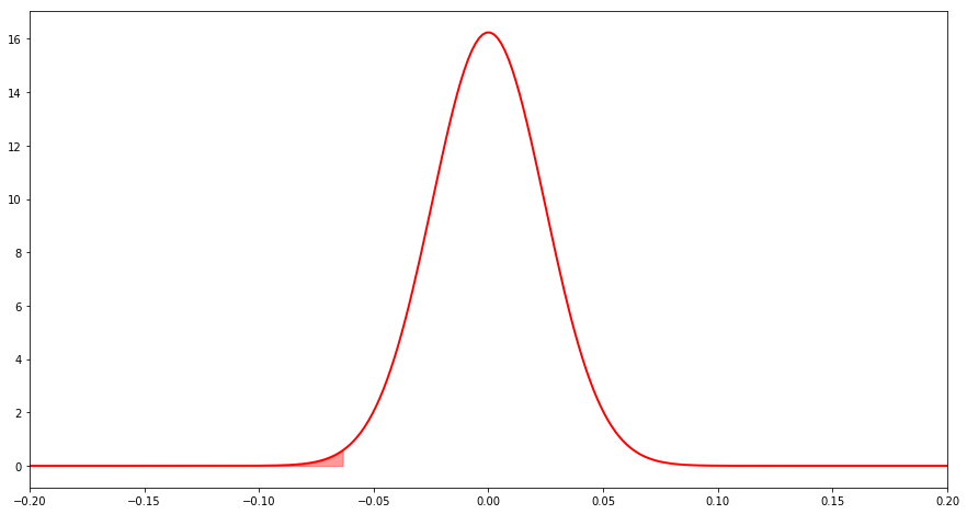
This is what we’d assume the distribution to look like under the conservative null hypothesis. If the difference is in the tails of this distribution, then we have sufficient evidence to reject the null.

joined_data = np.hstack([a_data, b_data])

shared_sample_prop = joined_data.mean()
shared_sample_var = (
    (
        (a_data.size + b_data.size)
        * shared_sample_prop
        * (1-shared_sample_prop)
    )
    / (a_data.size * b_data.size)
)

diff_dist = stats.norm(0, np.sqrt(shared_sample_var))

actual_diff_prop = a_data.mean() - b_data.mean()

print("Difference in sample proportions: {:.4f}".format(actual_diff_prop))

p_value = diff_dist.cdf(actual_diff_prop)
print("P-value for difference in sample proportions: {:.4f}".format(p_value))

Difference in sample proportions: -0.0633
P-value for difference in sample proportions: 0.0049

fig, ax = plt.subplots(figsize=(15, 8));

x = np.linspace(-0.2, 0.2, 250);
ax.plot(x, diff_dist.pdf(x), color='red', linewidth=2);
ax.fill_between(
    x, diff_dist.pdf(x), where=(x < actual_diff_prop),
    color='red', alpha=0.4
);
ax.set_xlim(-0.2, 0.2);

png

Result

It seems pretty clear that we have sufficient evidence to reject the null that the proportions are the same. Not only that we have enough evidence to reject the null that the frequency of A is greater than or equal to the frequency of B. Therefore, we can say that the frequency of A is probably less than that of B. How sure can we be? There’s a probability of less than 2.5% of observing an equal or more extreme result under the assumption of the null hypothesis that B is less than or equal to A.

There are also a lot of different assumptions that went into this. If we’d had fewer samples, we wouldn’t have been able to use the normal approximation for example.

Interpretation

The statistics speak is kind of confusing, but it’s necessary when doing this kind of A/B testing. One of the nice things about Bayes’ approach is that it’s much easier to interpret and understand.

Bayes

Using the exact same data how would we approach this using Bayesian testing?

I’m going to use the PyMC3 library to define a model. Using this model we can update our prior beliefs with new evidence (the data). We can then examine the posteriors to better understand the difference between A and B.

with pm.Model() as model:
    p_A = pm.Uniform("p_A", 0, 1)
    p_B = pm.Uniform("p_B", 0, 1)

    # Define the unknown deterministic delta
    # Previously we said that this was >= 0 under the null
    delta = pm.Deterministic('delta', p_A - p_B)

    # Results are 0 or 1, so bernoulli
    obs_A = pm.Bernoulli("obs_A", p_A, observed=a_data)
    obs_B = pm.Bernoulli('obs_B', p_B, observed=b_data)

    step = pm.Metropolis()
    trace = pm.sample(20000, step=step)
    burned_trace = trace[1000:]

100%|██████████| 20000/20000 [00:02<00:00, 7291.57it/s]

p_A_samples = burned_trace["p_A"]
p_B_samples = burned_trace["p_B"]
delta_samples = burned_trace["delta"]

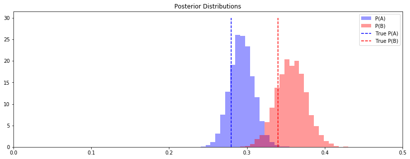
fig, ax = plt.subplots(figsize=(14, 5))

ax.set_xlim(0, 0.5)

ax.hist(
    p_A_samples, bins=np.linspace(0, 0.5, 80), color='blue',
    alpha=0.4, label="P(A)", normed=True
)
ax.vlines(
    p_A_true, 0, 30, linestyle='--', color='blue',
    label="True P(A)"
)
ax.hist(
    p_B_samples, bins=np.linspace(0, 0.5, 80), color='red',
    alpha=0.4, label="P(B)", normed=True
)
ax.vlines(
    p_B_true, 0, 30, linestyle='--', color='red',
    label="True P(B)"
)

ax.set_title("Posterior Distributions")
ax.legend();

png

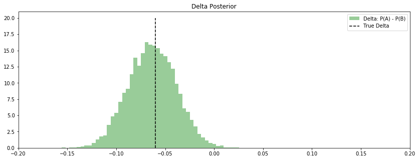
fig, ax = plt.subplots(figsize=(14, 5))

ax.set_xlim(-0.2, 0.2)

ax.hist(
    delta_samples, bins=50, color='green',
    label="Delta: P(A) - P(B)", normed=True, alpha=0.4
)
ax.vlines(
    p_A_true - p_B_true, 0, 20, linestyle='--',
    label="True Delta"
)
ax.set_title("Delta Posterior")
ax.legend();

png

Result

It’s pretty clear that the CTR on A is below that of B. How could we quantify this relationship? Just calculate the probability that delta is less than 0.

The interpretation of this result is really quite a bit simpler. The posteriors can just be seen as “belief”. Given all of your a prior assumptions and the evidence what is likely? The posteriors are an intuitive answer to this question.

print(
    "Proability that the CTR for A is less than B: {:.3f}"
    .format(np.mean(delta_samples < 0))
)

Proability that the CTR for A is less than B: 0.996