The Curse of Dimensionality

Intro

Many machine learning models rely on some distance metric to compute a measure of similarity in the feature space.

Sample problem

Given a sample density $\rho = \frac{n}{V}$, where $n$ is the number of uniformly distributed points and $V$ is the volume of the space those points occupy in $\mathbb{R}^3$, how many points $n$ are required in $\mathbb{R}^{10}$ in order to preserve the value of $\rho$?

Subpart 1: You’re not really able to use volume as it is in the formula, but you can figure out how volume scales with $n$ and that turns out to be enough. What’s the volume occupied by one point? How does volume scale as a function of n and dimension D?

$V = \frac{1}{n}^D$

Let’s say we hold volume constant and increase N. D must increase. If we increase the dimensionality D, then N must again increase at a rapid rate to maintain volume.

How many points in 10 dimensions, $n_{10}$, are required to have the same sample density in terms of the number of points in 3 dimensions, $n_3$?

Hover over box below to reveal the answer.

$n_{10} = n_3^\frac{10}{3}$

That’s a lot more points!

Derivation of Solution

$V \sim X^D$ where $V$ is volume, $X \in \mathbb{R}$, and $D \in \mathbb{I}$ is the integer dimension of the space.

Since we’re preserving $\rho$, we can just solve the equation for $n_{10}$ given $n_{3}$: $\rho_{3} = \rho_{10}$

Now, the key step using the assumption of uniform distribution. $\rho$ can be approximated as one over the volume occupied by 1 point. This gets us the most important takeaway which I already hinted at: $V = \frac{1}{n}^D \implies \rho \sim \frac{1}{n}^{-D}$

This relationship reflects how points become more distant as you increase the dimensionality under the assumption of uniform random distribution.

For example, imagine 2 points distributed in 1 dimension (a line). The average distance separating the points is 0.5. Therefore the density is 2; there’s one point for every half unit of space. Now, imagine adding a second dimension. The average x separation between the two points and the average y separation between the two points is still 0.5, but they now occupy an area, which is the square of their separation. The average separation has now become $\sqrt{\frac{1}{2}^2 + \frac{1}{2}^2} = \sqrt{\frac{1}{2}}$.

In the general case, if you have n points along a line that are uniformly distributed, the average distance between two points will be $\frac{1}{n}$. If you introduce another dimension, then that distance bumps up to $\frac{1}{n^{(1/2)}}$ and so on.

Substituting the previous result into the example problem yields:

$n_{10} = n_3^\frac{10}{3}$ .

This means the amount of data you need scales exponentially with more dimensions! And don’t make the mistake of thinking PCA solves this problem. It merely eliminates low variance variables even if they are significant! Ideally, one should test each variable independently to see if it’s useful and engineer fewer significant variables if need be.

Building intuition

Is there a way to visualize how point density changes with the addition of more dimensions?

import numpy as np

import matplotlib.pyplot as plt

import matplotlib.animation as animation

from scipy.linalg import block_diag

%matplotlib inline

Generating 100 points in 1 and 20 dimensions

n_points = 100

d1 = np.random.uniform(size=n_points)
d2 = np.random.uniform(size=(n_points, 2))
d3 = np.random.uniform(size=(n_points, 3))
d5 = np.random.uniform(size=(n_points, 5))
d10 = np.random.uniform(size=(n_points, 10))
d20 = np.random.uniform(size=(n_points, 10))

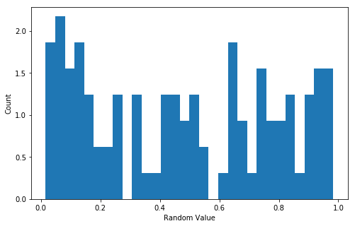
Histogram

The go-to way to visualize a one-dimensional distribution.

fig, ax = plt.subplots(figsize=(8,5))
ax.hist(d1, normed=True, bins=30);

ax.set_xlabel("Random Value");
ax.set_ylabel("Count");

png

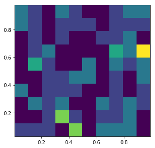
A 2D histogram

fig, ax = plt.subplots(figsize=(5, 5))

ax.hist2d(d2[:,0], d2[:,1], normed=True, bins=10);

png

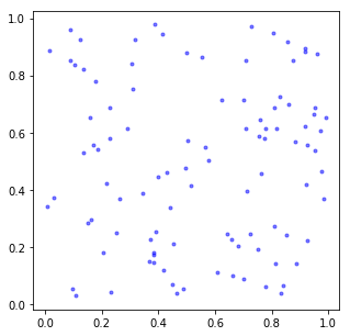
In this case a Scatterplot is a bit more illustrative because there are so few points.

fig, ax = plt.subplots(figsize=(5, 5))

ax.plot(d2[:,0], d2[:,1], 'b.', alpha=0.5);

png

Now, there’s a problem.

How do we deal with dimensions greater than 2 on a computer screen?

We can do what we always do–project the points from n-dimensional space into 2D space. Something else we can do is apply transformation matrices to the points–like rotation–to better visualize how far the points are from each other.

def get_rotation_matrix(dim, t):
    """Expects t to evolve over time for a full rotation
    Will always perform rotation in the same way along diagonal"""
    def one_rotation_matrix(t):
        return np.array(
            [[np.cos(t), -np.sin(t)],
            [np.sin(t), np.cos(t)]], dtype=float
        )

    first_arg = [np.identity(2)]
    if not dim % 2:
        block_args = (
            [one_rotation_matrix(t) for _ in range(dim / 2)]
        )
    else:
        blocks = dim // 2
        block_args = (
            [np.array([[1.]])]
            + [one_rotation_matrix(t) for _ in range(dim // 2)]
        )
    result = block_diag(*block_args)
    return result


def get_projection(data, t, proj_vector):
    """
    Inputs------
    data: a data array of shape (points, dimensions)
    t: a scalar which will be fed into a function for generating rotation
    transformation matrices
    proj_vector: The vector perpendicular to the plane onto which the points
    will be projected
    Outputs------
    Points in R2 after being transormed by rotation and projected onto the
    plane perpendicular to proj_vector
    """
    dim = data.shape[1]
    transformation = get_rotation_matrix(dim, t)
    proj_vector /= np.linalg.norm(proj_vector)
    points = transformation.dot(data.T).T
    return (points - (
        np.dot(points, proj_vector).reshape(points.shape[0], 1)
        * proj_vector.reshape(1, dim)
    ))[:, :2]


def get_originated_line_data(line_data):
    """
    Inputs--------
    line_data: An array of shape (points, dimensions(usually 2))
    Ouputs-------
    result: An array of shape (points * 2, dimensions)

    This function adds points representing the origin so matplotlib's
    default plot function will plot lines from the origin.
    (Other built-in mpl functions for this purpose aren't iterable.)
    """
    result = np.zeros((line_data.shape[0] * 2, line_data.shape[1]))
    for i in range(result.shape[0]):
        if i % 2 == 0:
            pass
        else:
            result[i, :] = line_data[i // 2, :]
    return result


def multid_plot(data, output_file='out.mp4'):
    """
    Create an animation of multi-dimensional data and save at output_fil
    """
    # Determine number of dimensions
    dim = data.shape[1]
    # Create array of orthonormal basis vectors
    line_data = np.identity(dim)
    # Find a random projection vector
    proj_vector = np.random.uniform(low=0.3, high=0.8, size=dim)

    # Grab first two columns
    X = data[:,:2]
    X_line = get_originated_line_data(line_data[:, :2])

    fig, ax = plt.subplots()
    ax.set_aspect('equal')
    ax.set_xlim(-2, 2)
    ax.set_ylim(-2, 2)


    scat, = ax.plot(
        X[:,0], X[:,1], 'b.'
    )
    line, = ax.plot(
        X_line[:, 0], X_line[:, 1], 'r'
    )

    def init():
        scat = ax.plot(
            X[:,0], X[:,1], 'b.'
        )
        line = ax.plot(line_data)
        return scat, line,

    def animate(t):
        t += (2 * np.pi) / 200.
        X = get_projection(data, t, proj_vector)
        X_line = get_originated_line_data(get_projection(line_data, t, proj_vector))
        scat.set_xdata(X[:, 0])
        scat.set_ydata(X[:, 1])
        line.set_data(X_line[:, 0], X_line[:, 1])
        return scat, line,

    anim = animation.FuncAnimation(
        fig, animate,
        frames=50, blit=False
    );
    anim.save(output_file, fps=5, extra_args=['-vcodec', 'libx264'])

Four dimensions

Five dimensions

Ten dimensions

Twenty dimensions

Notice anything?

With a higher number of dimensions, we start to notice that the points seem to jump around wildly. It isn’t because there’s more rotation. With each new frame, there’s an equivalent amount of rotation regardless of the number of dimensions–although more dimensions means we’re rotating around more axes.

Even though each point was chosen randomly somewhere from 0 to 1, the distances between points in higher dimensions is greater than it is in lower dimensions.

Euclidean distances

Measuring the distance between things is an important concept in a lot of fields. In the context of machine learning, distance between points can be used to determine some measure of their similarity (in some instances–in others cosine similarity or something else entirely may be appropriate).

What’s the distance between the origin and the midpoint of the higher dimensional space?

$\sqrt{D \times (0.5)^2}$

The general formula for euclidean distance between x and v is then the following:

$\sqrt{\Sigma_{i=0}^{D}{(x_i - v_i)^2}}$

In either case, it’s pretty clear that with more dimensions, distances increase.

How do we fix the curse?

This post was meant to show how the curse of dimensionality arises, but I discovered as I was working on it, it also starts to introduce one of the ways of coping with it: namely, projection. If there are more features than necessary, the best solution is also probably the easiest– just drop the useless stuff. If you don’t know what’s useful and what isn’t, projecting the data into a lower dimensional space may be fruitful. Which space specifically though is slightly more complicated to say. PCA helps one visualize things if one has no idea what to do, and linear discriminant analysis (LDA) is useful in classification problems.