Survival on the Titanic
A Hasty Attempt at the Titanic Kaggle Competition
Intro
Kaggle has hosted the titanic competition for a few years now. It gives aspiring data scientists the opportunity to test some basic classification approaches on a real dataset that’s familiar to almost anyone.
Motivation
My main goal with this attempt is to see how well I can do in a short amount of time. I’m not going to spend more than a day (or a few hours) on this in part becuase I think it seems kind of silly to try to eek out each bit of predictive power from the data when this is really just meant to be an interesting practice exercise.
from __future__ import division, print_function

# Basic imports. I'm using python 2

import numpy as np
import pandas as pd

import re

import seaborn as sns
import matplotlib.pyplot as plt

from sklearn.model_selection import (
    GridSearchCV, train_test_split, cross_val_score
)
from sklearn.ensemble import (
    AdaBoostClassifier, BaggingClassifier, GradientBoostingClassifier,
    RandomForestClassifier
)
from sklearn.svm import SVC
from sklearn.preprocessing import StandardScaler
from sklearn.pipeline import Pipeline

pd.set_option('display.max_columns', None)

%matplotlib inline
train = pd.read_csv('data/train.csv', index_col=0)
train.head()
| Survived | Pclass | Name | Sex | Age | SibSp | Parch | Ticket | Fare | Cabin | Embarked | |
|---|---|---|---|---|---|---|---|---|---|---|---|
| PassengerId | |||||||||||
| 1 | 0 | 3 | Braund, Mr. Owen Harris | male | 22.0 | 1 | 0 | A/5 21171 | 7.2500 | NaN | S |
| 2 | 1 | 1 | Cumings, Mrs. John Bradley (Florence Briggs Th... | female | 38.0 | 1 | 0 | PC 17599 | 71.2833 | C85 | C |
| 3 | 1 | 3 | Heikkinen, Miss. Laina | female | 26.0 | 0 | 0 | STON/O2. 3101282 | 7.9250 | NaN | S |
| 4 | 1 | 1 | Futrelle, Mrs. Jacques Heath (Lily May Peel) | female | 35.0 | 1 | 0 | 113803 | 53.1000 | C123 | S |
| 5 | 0 | 3 | Allen, Mr. William Henry | male | 35.0 | 0 | 0 | 373450 | 8.0500 | NaN | S |
<class 'pandas.core.frame.DataFrame'>
Int64Index: 891 entries, 1 to 891
Data columns (total 11 columns):
Survived    891 non-null int64
Pclass      891 non-null int64
Name        891 non-null object
Sex         891 non-null object
Age         714 non-null float64
SibSp       891 non-null int64
Parch       891 non-null int64
Ticket      891 non-null object
Fare        891 non-null float64
Cabin       204 non-null object
Embarked    889 non-null object
dtypes: float64(2), int64(4), object(5)
memory usage: 83.5+ KB
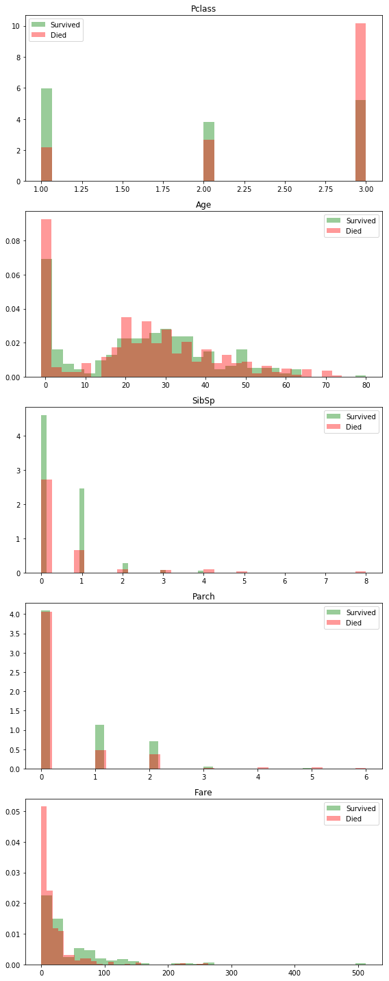
Feature Engineering
This is one of the most important and often overlooked parts of the modeling process. Unfortunately, as part of my effort to get respectable results as quickly as possible, I’m not going to spend as much time working on it either…
Rather than messing with my modeling approach, I could probably significantly improve my score by just making/using better, more predictive, features.
columns_to_investigate = ['Pclass', 'Age', 'SibSp', 'Parch', 'Fare']

fig, axes = plt.subplots(
    len(columns_to_investigate), 1, figsize=(8, 20)
)

survived_mask = (train['Survived'] == 1)

for ax, col in zip(axes, columns_to_investigate):
    ax.hist(
        train.loc[survived_mask, col].fillna(-1), bins=30,
        normed=True, color='g', label='Survived', alpha=0.4
    )
    ax.hist(
        train.loc[~survived_mask, col].fillna(-1), bins=30,
        normed=True, color='r', label='Died', alpha=0.4
    )
    ax.set_title(col)
    ax.legend()

fig.tight_layout()
Some Exploratory Histograms
Building a cleaning pipeline
title_re = re.compile(r' ([A-Za-z]+)\.')
title_replacements = {'Mlle': 'Miss', 'Ms': 'Miss', 'Mme': 'Mrs'}

cabin_letter_re = re.compile(r'([A-Z]+)')
cabin_num_re = re.compile(r'(\d+)')


def add_title_name_len(df):
    """
    Adds Title col astype int from Name
    Drops the name
    """
    df['Title'] = df['Name'].str.extract(title_re)
    df['Title'] = df['Title'].replace([
        'Lady', 'Countess','Capt', 'Col','Don', 'Dr', 'Major',
        'Rev', 'Sir', 'Jonkheer', 'Dona'
    ], 'Rare')
    df['Title'] = (
        df['Title']
        .map(title_replacements)
        .map({'Mr': 1, 'Miss': 2, 'Mrs': 3, 'Master': 4, 'Rare': 5})
        .fillna(0)
        .astype(int)
    )
    df['NameLen'] = df['Name'].str.len()
    df.drop('Name', axis=1, inplace=True)

def clean_sex(df):
    """self-explanatory"""
    df['Sex'] = df['Sex'].fillna(df['Sex'].mode())
    df['Sex'] = df['Sex'].map({'female': 0, 'male': 1})

def add_family_size(df):
    df['FamilySize'] = df['SibSp'] + df['Parch']

def classify_ages(df):
    """
    Adds MissingAge column
    Makes Age an int column with categories from 1 to 5 ordered by age
    """
    age_cuts = [15, 20, 30, 40, 50, 60]
    df['MissingAge'] = 0.
    df.loc[(df['Age'].isnull()), 'MissingAge'] = 1.
    df['Age'] = pd.cut(
        df['Age'], bins=age_cuts, labels=range(1, len(age_cuts))
    ).astype(float)
    df['Age'] = df['Age'].fillna(0).astype(int)

def clean_fare(df):
    """
    Adds a MissingFare column
    Fills missing fares with 0s
    Adds a quantile for fare
    """
    cuts = [4, 7, 10, 20, 50, 100, 200]
    # Don't expect this to be missing
    df['Fare'] = df['Fare'].fillna(0)
    df['QuantFare'] = pd.cut(
        df['Fare'], cuts, labels=range(1, len(cuts))
    ).astype(float)

def clean_embarked(df):
    """
    Fill the very few missing with mode
    Maps to integers
    """
    df['Embarked'] = df['Embarked'].fillna(df['Embarked'].mode())
    df['Embarked'] = (
        df['Embarked']
        .fillna(df['Embarked'].mode()[0])
        .map({'S': 0, 'C': 1, 'Q': 2}).astype(int)
    )

def clean_cabin(df):
    """
    Adds MissingCabin column
    Adds a CabinLetter column with letters mapped to ints
    Adds a CabinNumber column of type ints
    Drops original Cabin column
    """
    df['MissingCabin'] = 0
    df.loc[df['Cabin'].isnull(), 'MissingCabin'] = 1
    df.loc[df['Cabin'].isnull(), 'Cabin'] = ''
    df['CabinLetter'] = (
        df['Cabin'].str.extract(cabin_letter_re).fillna('')
    )
    df['CabinNumber'] = (
        df['Cabin'].str.extract(cabin_num_re)
        .astype(float)
        .fillna(0)
        .astype(int)
    )
    df.drop('Cabin', axis=1, inplace=True)

def categorize(df, columns):
    """
    Given a df and list of columns, converts those columns to dummies
    concats them with the df and drops the original columns.
    """
    for col in columns:
        dummy_df = pd.get_dummies(df[col], prefix=col, drop_first=True)
        df.drop(col, axis=1, inplace=True)
        df = pd.concat([df, dummy_df], axis=1)
    return df

def data_prep(df):
    add_title_name_len(df)
    clean_sex(df)
    classify_ages(df)
    add_family_size(df)
    df.drop('Ticket', axis=1, inplace=True)
    clean_fare(df)
    # On second thought, try dropping this. There's not reason to think it's predictive
#     clean_embarked(df)
    df.drop('Embarked', axis=1, inplace=True)
    clean_cabin(df)
    return categorize(df, ['Title', 'Age', 'QuantFare', 'CabinLetter'])
train = pd.read_csv('data/train.csv', index_col=0)
train = data_prep(train)
train.head()
| Survived | Pclass | Sex | SibSp | Parch | Fare | NameLen | MissingAge | FamilySize | MissingCabin | CabinNumber | Title_2 | Title_3 | Age_1 | Age_2 | Age_3 | Age_4 | Age_5 | QuantFare_2.0 | QuantFare_3.0 | QuantFare_4.0 | QuantFare_5.0 | QuantFare_6.0 | CabinLetter_A | CabinLetter_B | CabinLetter_C | CabinLetter_D | CabinLetter_E | CabinLetter_F | CabinLetter_G | CabinLetter_T | |
|---|---|---|---|---|---|---|---|---|---|---|---|---|---|---|---|---|---|---|---|---|---|---|---|---|---|---|---|---|---|---|---|
| PassengerId | |||||||||||||||||||||||||||||||
| 1 | 0 | 3 | 1 | 1 | 0 | 7.2500 | 23 | 0.0 | 1 | 1 | 0 | 0 | 0 | 0 | 1 | 0 | 0 | 0 | 1 | 0 | 0 | 0 | 0 | 0 | 0 | 0 | 0 | 0 | 0 | 0 | 0 |
| 2 | 1 | 1 | 0 | 1 | 0 | 71.2833 | 51 | 0.0 | 1 | 0 | 85 | 0 | 0 | 0 | 0 | 1 | 0 | 0 | 0 | 0 | 0 | 1 | 0 | 0 | 0 | 1 | 0 | 0 | 0 | 0 | 0 |
| 3 | 1 | 3 | 0 | 0 | 0 | 7.9250 | 22 | 0.0 | 0 | 1 | 0 | 0 | 0 | 0 | 1 | 0 | 0 | 0 | 1 | 0 | 0 | 0 | 0 | 0 | 0 | 0 | 0 | 0 | 0 | 0 | 0 |
| 4 | 1 | 1 | 0 | 1 | 0 | 53.1000 | 44 | 0.0 | 1 | 0 | 123 | 0 | 0 | 0 | 0 | 1 | 0 | 0 | 0 | 0 | 0 | 1 | 0 | 0 | 0 | 1 | 0 | 0 | 0 | 0 | 0 |
| 5 | 0 | 3 | 1 | 0 | 0 | 8.0500 | 24 | 0.0 | 0 | 1 | 0 | 0 | 0 | 0 | 0 | 1 | 0 | 0 | 1 | 0 | 0 | 0 | 0 | 0 | 0 | 0 | 0 | 0 | 0 | 0 | 0 |
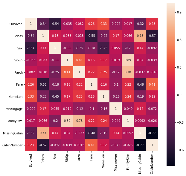
Predictor Correlations
plt.figure(figsize=(10, 10));

sns.heatmap(train.iloc[:, :11].corr(), square=True, annot=True);
Investigating Feature Usefulness
mini_df = train.iloc[:, :10].copy()

columns_to_investigate = mini_df.columns[1:10]

fig, axes = plt.subplots(9, 1, figsize=(10, 30))

survived_mask = (mini_df['Survived'] == 1)

for i, (col, ax) in enumerate(zip(columns_to_investigate, axes)):
#     print(i, col, ax)
    ax.hist(
        mini_df.loc[survived_mask, col], bins=30,
        normed=True, color='g', label='Survived', alpha=0.4
    )
    ax.hist(
        mini_df.loc[~survived_mask, col], bins=30,
        normed=True, color='r', label='Died', alpha=0.4
    )
    ax.set_title(col)
    ax.legend()
fig.tight_layout()
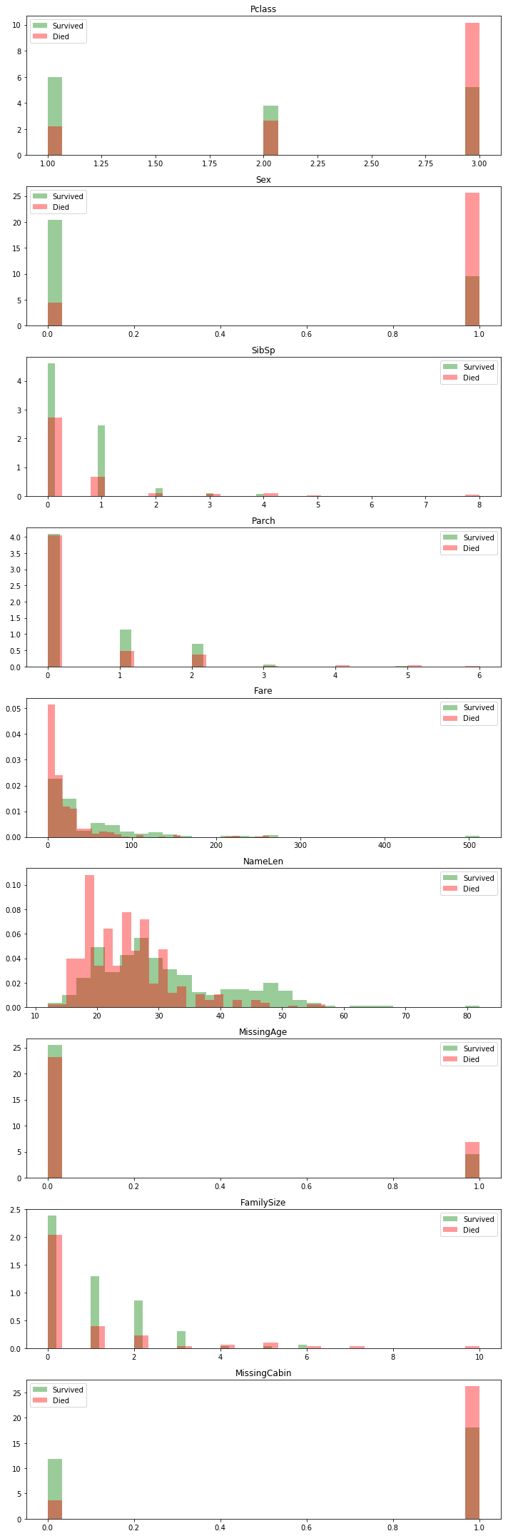
One thing of note: missing data seems to almost always be a bad sign. It’s probably correlated with wealth in some way since the lower class “less important” individuals are probably less likely to have complete information available.
y_train = train.pop('Survived').values
X_train = train.values
Parameter selection via grid search CV
I’m going to try out the following models:
- RandomForestClassifier
- AdaBoostClassifier
- BaggingClassifier
- GradientBoostingClassifier
- SupportVectorClassifier
Of course by fitting all of these hyperparameters to the training data, I run the risk of starting to meta overfit the training data by overtuning the hyperparameters to just the training data. That’s not something I’m particularly worried about with this project though.
Generally in cases where there is a n_estimators parameter, I use a low learning rate with a larger number of estimators or iterations to limit the risk of overfitting.
# A running dictionary of all my models, so I can keep track of everything
all_ensembles = dict()
Random Forest
rfc = RandomForestClassifier()

rfc_param_grid = {
    'n_estimators': [500],
    'max_features': np.arange(3, 7, 1, dtype=int),
    'min_samples_split': [4, 5, 6]
}

rfc_g = GridSearchCV(
    rfc, rfc_param_grid, scoring='accuracy', cv=5, n_jobs=-1, verbose=1
)
rfc_g.fit(X_train, y_train)
print(rfc_g.best_score_)

print(rfc_g.best_params_)
0.810325476992
{'max_features': 3, 'min_samples_split': 6, 'n_estimators': 500}
rf_model = RandomForestClassifier(
    n_estimators=3000, max_features=3, min_samples_split=6
)

rf_scores = (
    cross_val_score(
        rf_model, X_train, y_train, scoring='accuracy', verbose=1, n_jobs=-1
    )
)
rf_score = rf_scores.mean()
print(rf_score)
# 0.828

rf_model.fit(X_train, y_train)
all_ensembles.update({'rf': (rf_model, rf_score)})
AdaBoost Classifier
abc = AdaBoostClassifier()

abc_param_grid = {
    'n_estimators': [1000],
    'learning_rate': [0.01, 0.1, 0.3]
}

abc_g = GridSearchCV(
    abc, abc_param_grid, scoring='accuracy', cv=5, n_jobs=-1, verbose=1
)
abc_g.fit(X_train, y_train)
print(abc_g.best_score_)
# 0.801346

print(abc_g.best_params_)
# {'learning_rate': 0.1, 'n_estimators': 1000}
abc_model = AdaBoostClassifier(
    n_estimators=2000, learning_rate=0.1
)

# Past 1500 estimators doesn't help as much here

abc_scores = (
    cross_val_score(
        abc_model, X_train, y_train, scoring='accuracy', verbose=1, n_jobs=-1
    )
)
abc_score = abc_scores.mean()
print(abc_score)
# 0.795

abc_model.fit(X_train, y_train)
all_ensembles.update({'abc': (abc_model, abc_score)})
Bagging
bag = BaggingClassifier()

bag_param_grid = {
    'base_estimator': [None],
    'n_estimators': [10, 25, 30, 40],
    'max_samples': [0.2, 0.3, 0.5, 0.7, 1.],
    'max_features': [0.95, 1.]
}

bag_param = GridSearchCV(
    bag, bag_param_grid, scoring='accuracy', n_jobs=-1, cv=5,
    verbose=1
)
bag_param.fit(X_train, y_train)
print(bag_param.best_score_)
# 0.8226

print(bag_param.best_params_)
# {'base_estimator': None,
#  'max_features': 0.95,
#  'max_samples': 0.5,
#  'n_estimators': 25}
bag_model = BaggingClassifier(
    n_estimators=25, max_features=1., max_samples=0.3
)

bag_scores = (
    cross_val_score(
        bag_model, X_train, y_train, scoring='accuracy', verbose=1, cv=5
    )
)
bag_score = bag_scores.mean()
print(bag_score)
# 0.802

bag_model.fit(X_train, y_train)
all_ensembles.update({'bagging': (bag_model, bag_score)})
GradientBoosting
gb_classifier = GradientBoostingClassifier()

gb_param_grid = {
    'learning_rate': [0.1],
    'n_estimators': [3000],
    'max_depth': [3, 5, 7],
    'subsample': [0.5, 0.75, 1]
}

gb_param = GridSearchCV(
    gb_classifier, gb_param_grid, scoring='accuracy', n_jobs=-1, cv=5,
    verbose=1
)
gb_param.fit(X_train, y_train)
print(gb_param.best_score_)
# 0.82267

print(gb_param.best_params_)
# {'learning_rate': 0.1, 'max_depth': 7, 'n_estimators': 3000, 'subsample': 0.5}
gb_model = GradientBoostingClassifier(
    learning_rate=0.1, max_depth=7, n_estimators=3000, subsample=0.95
)
gb_scores = (
    cross_val_score(
        gb_model, X_train, y_train, scoring='accuracy', verbose=1, cv=5, n_jobs=-1
    )
)
gb_score = gb_scores.mean()
print(gb_score)
# 0.80

gb_model.fit(X_train, y_train)
all_ensembles.update({'gb': (gb_model, gb_score)})
Support Vector Machine Classifier
svc = SVC()

svc_pipe = Pipeline([
    ('scale', StandardScaler()),
    ('svc', svc)
])


svc_grid_params = [{
        'svc__kernel': ['poly'],
        'svc__degree': np.arange(1, 8, dtype=int),
        'svc__C': np.logspace(-2, 3, 8)
    },
    {
        'svc__kernel': ['rbf'],
        'svc__gamma': np.logspace(-4, 2, 8),
        'svc__C': np.logspace(-2, 2, 10)
    }
]

svc_grid = GridSearchCV(
    svc_pipe, param_grid=svc_grid_params, n_jobs=-1,
    verbose=2
)
svc_grid.fit(X_train, y_train)
print(svc_grid.best_score_)
# 0.818

print(svc_grid.best_params_)
# {'svc__C': 1.6681005372000592,
#  'svc__gamma': 0.26826957952797248,
#  'svc__kernel': 'rbf'}
svc_model = SVC(
    C=30., kernel='rbf', gamma=0.005
)

svc_scores = (
    cross_val_score(
        svc_model, X_train, y_train, scoring='accuracy', verbose=1, cv=5
    )
)

svc_score = svc_scores.mean()
print(svc_score)
# 0.773
svc_model.fit(X_train, y_train)

all_ensembles.update({'svc': (svc_model, svc_score)})
XGBoost
import xgboost as xgb
X_train1, X_test1, y_train1, y_test1 = train_test_split(X_train, y_train)
def add_empty_missing_cols(df, all_columns):
    for col in all_columns:
        if col not in df.columns and col != 'Survived':
            df[col] = 0.
    return df

# Preparing the test data
test = pd.read_csv('data/test.csv', index_col=0)
test = data_prep(test)
test = add_empty_missing_cols(test, train.columns)

X_test = test.values
xgb_model = xgb.XGBClassifier(
    max_depth=3, n_estimators=3000, learning_rate=0.005
)
xgb_score = cross_val_score(xgb_model, X_train, y_train).mean()
print(xgb_score)
# On mini test from within training
# 0.8226
all_ensembles.update({'xgb': (xgb_model, xgb_score)})
xgb_model.fit(X_train, y_train)

y_test_pred = xgb_model.predict(X_test)

final_results = pd.DataFrame(
    {'PassengerId': test.index.values, 'Survived': y_test_pred}
)

final_results.head()
| PassengerId | Survived | |
|---|---|---|
| 0 | 892 | 0 |
| 1 | 893 | 1 |
| 2 | 894 | 0 |
| 3 | 895 | 0 |
| 4 | 896 | 1 |
final_results.to_csv('data/final_result.csv', index=False)

# Got a 76 on the Kaggle submission
Ensembling
def ultra_ensembled_model(fit_estimators, X):
    """
    This isn't really serious, but it will be interesting to see how
    it does.
    """
    score_normalization = np.sum([v[1] for v in fit_estimators.values()])
    predictions = np.zeros((X.shape[0], len(fit_estimators)))
    for i, (name, (estimator, score)) in enumerate(fit_estimators.iteritems()):
        weight = score / score_normalization
        try:
            predictions[:, i] = estimator.predict(X) * weight
        except:
            print("ERROR:", name)
    return (predictions.sum(axis=1) > 0.5).astype(int)
y_pred = ultra_ensembled_model(all_ensembles, X_train)

acc = (y_pred == y_train).sum() / y_pred.size

print("Accuracy:", acc)

# Accuracy: 0.90
# This is on the training data, which is what it was fit to, so there's
# probably a lot of overfitting
y_test_pred = ultra_ensembled_model(all_ensembles, X_test)

final_results = pd.DataFrame(
    {'PassengerId': test.index.values, 'Survived': y_test_pred}
)
final_results.head()
| PassengerId | Survived | |
|---|---|---|
| 0 | 892 | 0 |
| 1 | 893 | 1 |
| 2 | 894 | 0 |
| 3 | 895 | 0 |
| 4 | 896 | 1 |
Conclusion
In the end, my best score was from the ensemble, where I got a score of 78%. While I do think it’s possible to improve that, it will most likely involve a lot of time sitting and thinking really carefully about feature engineering–which obviously isn’t possible in a short amount of time.
How are people getting >90% accuracy?
I’m extremely skeptical of the submissions in which people get accuracies of anything greater than ~85-90%. It just doesn’t seem remotely possible to be able to predict whether someone would live or die that night only on the basis of their income/class, gender, age, and name with that much accuracy. There are just too many other factors at play. Any score that high was achieved by other means (i.e. fitting the test data through repeated submissions).