Fractals
Animated Fractals with Matplotlib
Background and Motivation
Fractals are patterns exhibiting self-similar forms. This is also referred to as expanding symmetry.
Another interesting characteristic of fractals are their dimensionality. A typical polygon’s (e.g. a rectangle) area scales with the square of its length, so it has a dimension of 2. We’re used to integer dimensions. Fractal areas scale with a different factor, often denoted $D$ and more precisely known as the Hausdorff dimension, which can be non-integer.
Why?
As is often the case in mathematics, fractals may seem to be a useless abstraction, but they actually have significant real-world utility in tons of fields. Chaotic, dynamical systems– even something as simple as a double pendulum–can be modeled with differential equations, whose solutions exhibit extreme sensitivity to initial conditions. Despite the chaotic nature of many of these problems, there’s extreme utility to studying what solutions look like. I also wanted to create some new images for banners on my blog!
The Mandelbrot Set Defined
One way to generate fractal structures is by the iteration of functions in the complex number plane.
The formal definition of the Mandelbrot set is fairly short:
The Mandelbrot set consists of values ($c$) in the complex plane for which the orbit of 0 under iteration of the mapping: remains bounded.
In other words, it consists of any complex value $c$ that when plugged into the formula above with the starting value of $z_n=0$ iteratively, the absolute value of of $z_n$ remains bounded.
Another representation of the same thing in possibly more compact notation is the following:
Sources:
- Wikipedia has a lot of good info about the mandelbrot set.
- I also highly recommend the book Fractals, Chaos, and Power Laws.
# Just some imports (I used python2.7)

from __future__ import division

import numpy as np

import matplotlib as mpl
# mpl.verbose.set_level("helpful")

from matplotlib import pyplot as plt
from matplotlib import animation
from matplotlib import colors

from IPython.display import HTML

plt.rcParams['animation.html'] = 'html5'

%matplotlib inline
Python definition
Let’s define a simple mandelbrot set function in python that will take a real and imaginary component of a complex number (or x and y) and return a boolean that indicates whether the value of $z_n$ doesn’t diverge given a horizon of 2.0.
def is_mandelbrot(x, y, maxiter=100, horizon=2.0):
    """
    Given float x (real) and float y (imaginary)
    returns bool indicating if the value is in the mandelbrot set
    """
    c = x + y * 1j
    zn = 0.0 # initialize z_n to 0
    for n in range(maxiter):
        zn = zn ** 2 + c
    return abs(zn) < horizon

# now test it out on a point that we know that should be outside
is_mandelbrot(0.274,0.482, maxiter=200)  # Returns False
# Extend the definition to work with numpy arrays which will make things way faster through
# vectorization

def mandelbrot_set(xmin, xmax, ymin, ymax, xn, yn, maxiter, horizon=2.0):
    """
    Inputs:
        xmin/xmax: min/max real component
        ymin/ymax: min/max imag component
        xn/yn: number of x/y values to test
        maxiter: Number of iterations
    """
    X = np.linspace(xmin, xmax, xn, dtype=np.float32)
    Y = np.linspace(ymin, ymax, yn, dtype=np.float32)
    C = X + Y[::-1, None] * 1j
    N = np.zeros(C.shape, dtype=int)
    Z = np.zeros(C.shape, np.complex64)
    for n in range(maxiter):
        I = np.less(abs(Z), horizon)
        N[I] = n
        Z[I] = Z[I]**2 + C[I]
    N[N == maxiter-1] = 0
    return Z, N
# Setting up some constants
xn = 2560
yn = 0.625 * xn

dpi = 300
width = 2560 / dpi
height = np.floor(width * yn / xn)

maxiter = 300
horizon = 2.0 ** 40
log_horizon = np.log(np.log(horizon))/np.log(2)
def plot_mandelbrot(xmin, xmax, ymin, maxiter = 300):
    """
    Plots mandelbrot

    Inputs: x_min, x_max, y_min, (y_max is determined from xn, yn, and other variables)
    Requires variables in namespace:
    xn, yn, dpi, width, height, horizon, log_horizon
    """
    ymax = ymin + (xmax - xmin) * 0.625

    Z, N = mandelbrot_set(xmin, xmax, ymin, ymax, xn, yn, maxiter, horizon)

    with np.errstate(invalid='ignore'):
        M = np.nan_to_num(N + 1 -
                          np.log(np.log(abs(Z)))/np.log(2) +
                          log_horizon)

    fig = plt.figure(figsize=(width, height), dpi=dpi)
    ax = fig.add_axes([0.0, 0.0, 1.0, 1.0], frameon=False, aspect=1)

    # rendering
    M = (
        colors.LightSource(azdeg=315, altdeg=10)
        .shade(
            M, cmap=plt.cm.magma,
            norm=colors.PowerNorm(gamma=0.9), blend_mode='overlay'
        )
    )
    plt.imshow(M, interpolation="bicubic")
    ax.set_xticks([])
    ax.set_yticks([])
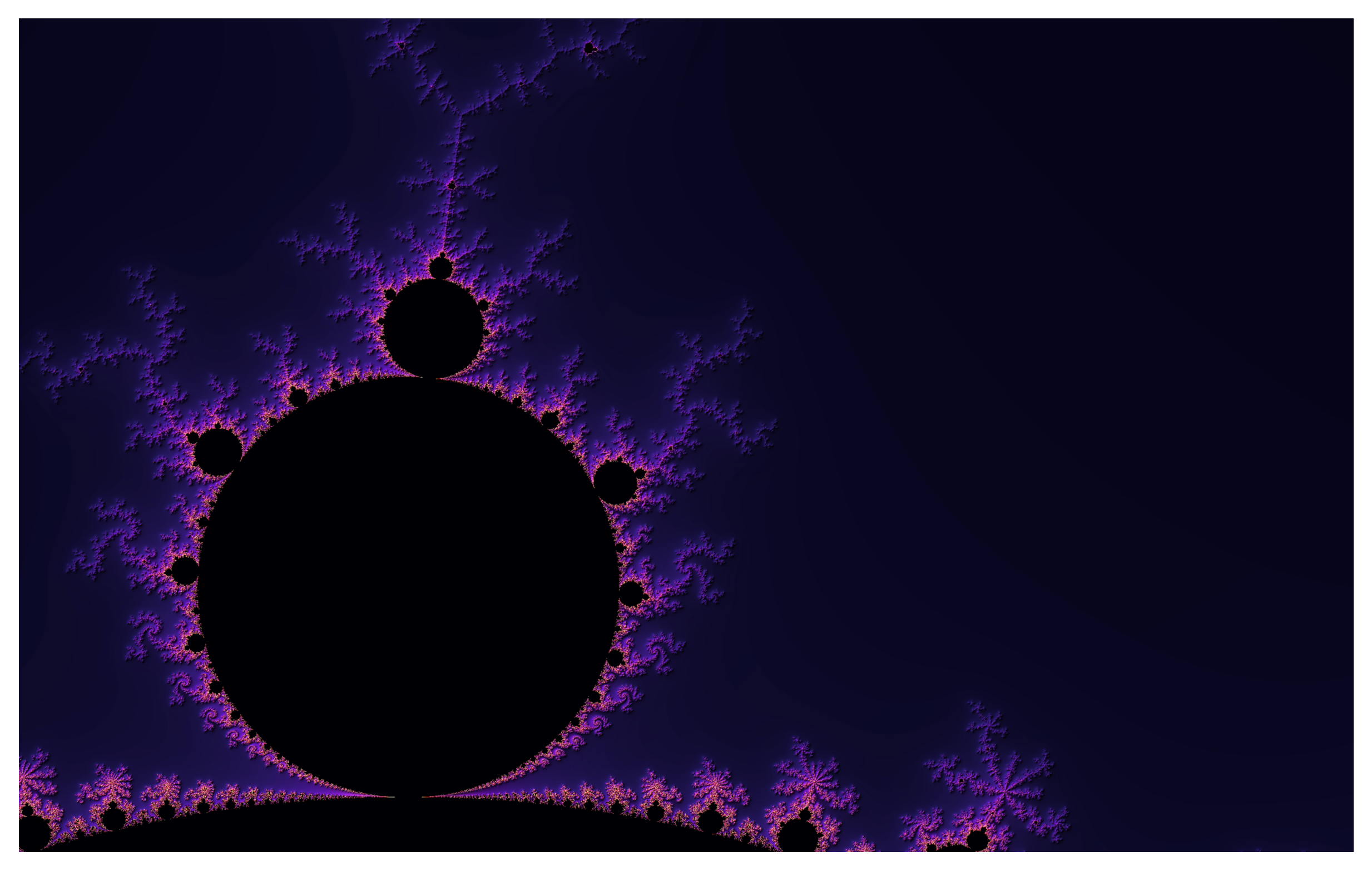
xmin, xmax = -0.3, +0.3
# ymin, ymax = +0.625, +1
ymin = +0.625

plot_mandelbrot(xmin, xmax, ymin)

# In case you're following along and would like to save plots...
# plt.savefig('images/mandelbrot_zoom.png')

plt.show()
# It seems to work!
# Let's check out a few more regions
# 0.274,0.482
# -0.088,0.654
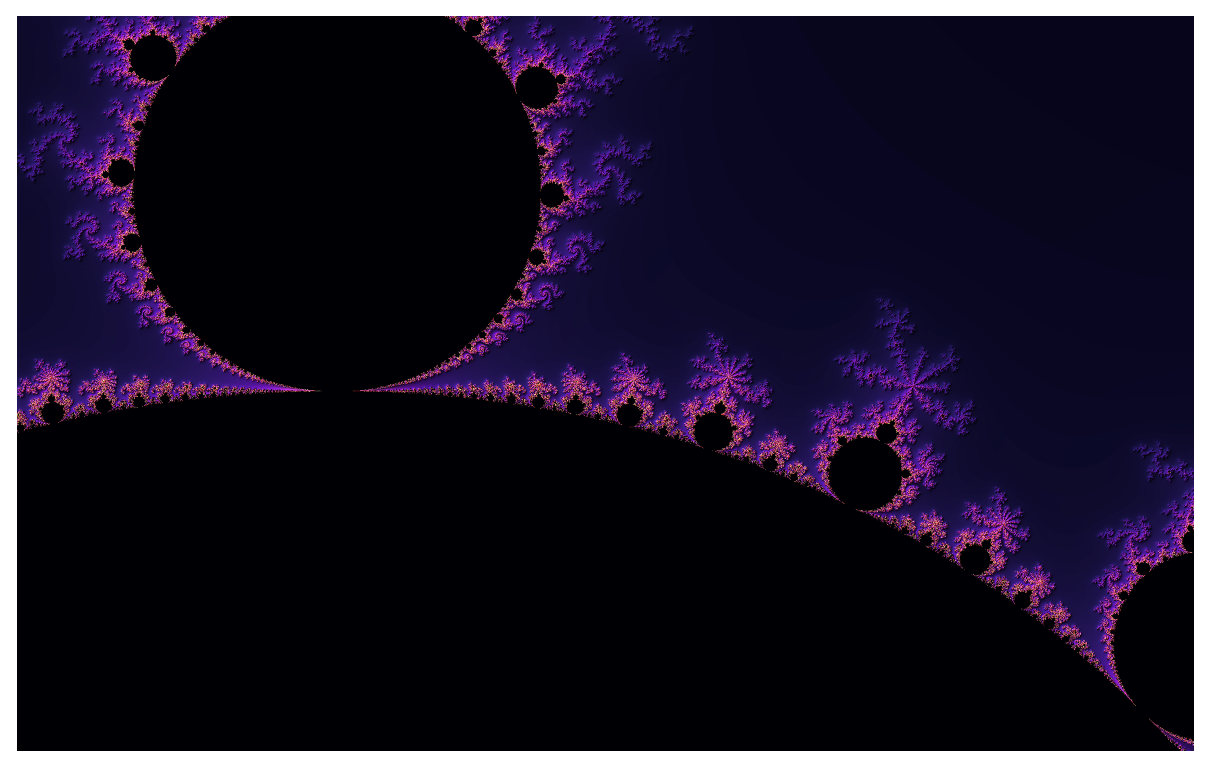
xmin, xmax = -0.273999, +0.274001
ymin = +0.481999
plot_mandelbrot(xmin, xmax, ymin, maxiter=300)
# plt.savefig('images/mandelbrot_zoom.png')
plt.show()
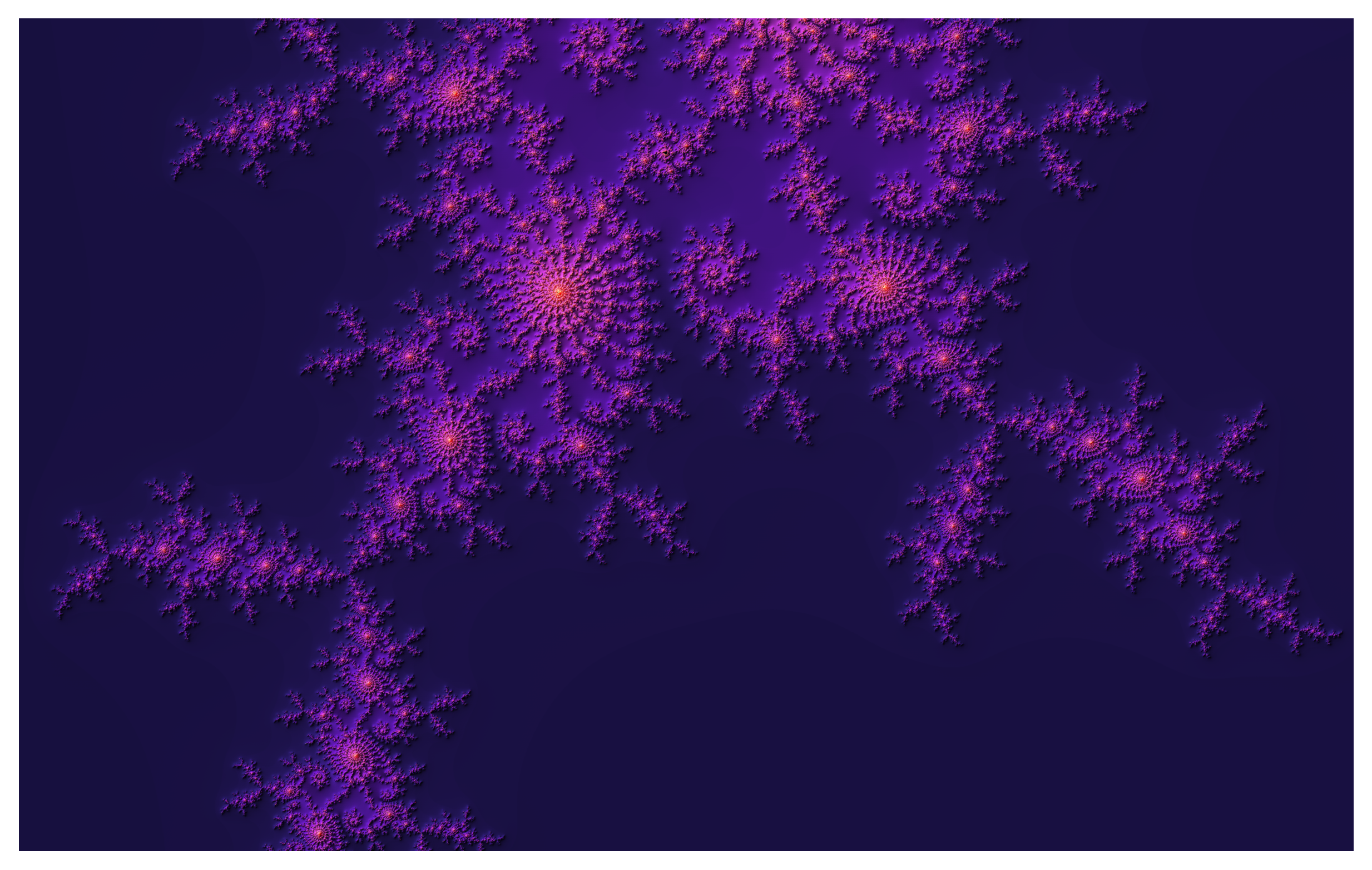
# -0.1002,0.8383
xmin, xmax = -0.1003, -0.1008
ymin = +0.8381

plot_mandelbrot(xmin, xmax, ymin, maxiter=800)

# plt.savefig('images/mandelbrot_zoom_2.png')

plt.show()
Animation
There are two interesting candidates for animation:
- How does the boundary evolve as we increase the number of iterations towards infinity?
- Changing x and y limits to zoom into interesting regions
We can modify the existing code to now produce an animation.
Animating as $Z_n$ approaches $\infty$
# Trying number 1 first

# Constants
xn = 2560
yn = 1600

# lower and upper bounds
# This region was painstakingly identified as extra delicious
xmin, xmax = -0.3, +0.3
ymin, ymax = +0.625, +1

maxiter = 2

maxiter_increment = 1

dpi = 100  # Adjust this depending on the resolution you want

width = 300 / dpi
height = width * yn / xn

horizon = 2.0 ** 40
log_horizon = np.log(np.log(horizon))/np.log(2)


def im_function(maxiter):
    Z, N = mandelbrot_set(xmin, xmax, ymin, ymax, xn, yn, maxiter, horizon)
    with np.errstate(invalid='ignore'):
        M = np.nan_to_num(
            N + 1 - np.log(np.log(abs(Z))) / np.log(2) + log_horizon
        )
    # rendering
    M = (
        colors.LightSource(azdeg=315, altdeg=10)
        .shade(
            M, cmap=plt.cm.magma,
            norm=colors.PowerNorm(gamma=0.9), blend_mode='overlay'
        )
    );
    return M


def updatefig(*args):
    global maxiter
    maxiter += maxiter_increment
    im.set_array(im_function(maxiter));
    return im,


# Start the figure up
fig = plt.figure(figsize=(width, height), dpi=dpi);
ax = fig.add_axes([0.0, 0.0, 1.0, 1.0], frameon=False, aspect=1);


im = plt.imshow(
    im_function(maxiter),
    interpolation="bicubic"
);

ani = animation.FuncAnimation(fig, updatefig, frames=40, blit=True);

ax.set_xticks([]);
ax.set_yticks([]);

HTML(ani.to_html5_video())
# ani.save('mandelbrot_iterations.mp4', fps=15, extra_args=['-vcodec', 'libx264'])
Animating a zoom
# Constants
xn = 2560
yn = 1600

# start lower and upper bounds
# xmin, xmax = -0.1003, -0.1008
# ymin, ymax = 0, +1.6
xmin, xmax = -3, 2.798899
ymin = -0.8

maxiter = 100

# xfocus, yfocus = (-0.1002, 0.8383)
zoom_factor_frame = 0.90

dpi = 400
width = 300 / dpi
height = width * yn / xn

horizon = 2.0 ** 40
log_horizon = np.log(np.log(horizon))/np.log(2)


def im_function(xmin, xmax, ymin, ymax, maxiter=maxiter):
    Z, N = mandelbrot_set(xmin, xmax, ymin, ymax, xn, yn, maxiter, horizon)
    with np.errstate(invalid='ignore'):
        M = np.nan_to_num(
            N + 1 - np.log(np.log(abs(Z))) / np.log(2) + log_horizon
        )
    # rendering
    M = (
        colors.LightSource(azdeg=315, altdeg=10)
        .shade(
            M, cmap=plt.cm.magma,
            norm=colors.PowerNorm(gamma=0.9), blend_mode='overlay'
        )
    );
    return M


def get_new_ranges_pan(xmin, xmax, ymin):
    def is_close(mid, foc, diff=0.001):
        return abs(mid - foc) < diff

    old_xrange = (xmax - xmin)
    old_yrange = (ymax - ymin)
    new_xrange = old_xrange * zoom_factor_frame
    new_yrange = old_yrange * zoom_factor_frame
    x_midpoint = (xmin + (old_xrange / 2))
    y_midpoint = (ymin + (old_yrange / 2))

    if is_close(x_midpoint, xfocus) and is_close(y_midpoint, yfocus):
        xdiff = old_xrange - new_xrange
        ydiff = old_yrange - new_yrange
        xmin = xmin + (xdiff / 2)
        xmax = xmax - (xdiff / 2)
        ymin = ymin + (ydiff / 2)
        ymax = ymax - (ydiff / 2)
    elif x_midpoint < xfocus and y_midpoint < yfocus:
        # midpoint of image is lower left of focus, zoom while hugging lower left
        # xmax and ymax are unchanged
        xmin = xmax - new_xrange
        ymin = ymax - new_yrange
    elif x_midpoint < xfocus and y_midpoint > yfocus:
        xmin = xmax - new_xrange
        ymax = ymin + new_yrange
    elif x_midpoint > xfocus and y_midpoint < yfocus:
        xmax = xmin + new_xrange
        ymin = ymax - new_yrange
    elif x_midpoint > xfocus and y_midpoint > yfocus:
        xmax = xmin + new_xrange
        ymax = ymin + new_yrange

    return xmin, xmax, ymin, ymax

def get_new_range(xmin, xmax, ymin):
    ymax = ymin + (xmax - xmin) * 0.625
    old_xrange = (xmax - xmin)
    old_yrange = (ymax - ymin)
    new_xrange = old_xrange * zoom_factor_frame
    new_yrange = old_yrange * zoom_factor_frame
    xdiff = (old_xrange - new_xrange) / 2
    ydiff = (old_yrange - new_yrange) / 2
    return xmin+xdiff, xmax-xdiff, ymin+ydiff, ymax-ydiff


def updatefig(*args):
    global xmin, xmax, ymin, ymax
    xmin, xmax, ymin, ymax = get_new_range(xmin, xmax, ymin)
    im.set_array(im_function(xmin, xmax, ymin, ymax, maxiter));
    return im,


# Start the figure up
fig = plt.figure(figsize=(width, height), dpi=dpi);
ax = fig.add_axes([0.0, 0.0, 1.0, 1.0], frameon=False, aspect=1);


im = plt.imshow(
    im_function(xmin, xmax, ymin, ymax, maxiter),
    interpolation="bicubic"
);

ani = animation.FuncAnimation(fig, updatefig, frames=30, blit=True);

ax.set_xticks([]);
ax.set_yticks([]);

# ani.save('mandelbrot_zoom.mp4', fps=15, extra_args=['-vcodec', 'libx264']);

HTML(ani.to_html5_video())
# plt.show()
One last interesting tidbit
Hilbert Curve
A Hilbert Curve is a continuous 1-D fractal curve that fills up a 2-D space. See the wiki. Despite the fact that it’s a one-dimensional line, it has dimension of two. The location of any point located in the unit square $(x, y)$ can be encoded as $d$ the distance along the Hilbert surface (there are also equivalents in higher dimensions).
Points that are local along the Hilbert surface in $\mathbb{R}$ must also necessarily be local in $\mathbb{R}^2$, but the converse is not always true.
This gives one the ability to map from 2D to 1D, but not the reverse ability.
Coming up next…
A mapping that’s much better behaved (i.e., it has an inverse) and has widespread use in statistics and machine learning. It’s the kernel.